---

Model Types

We have developed two modeling types to simulate traffic behavior. Each type realistically simulates conditions found in the field using \(t-x\) trajectories as the principle means of comparison. The models are fundamentally different. One is a deterministic model and the other is a stochastic model. The forecasts from the two models compliment one another. Both satisfy the principal aim of developing the cartools package: To explain highway performance as simply as possible, two model structures have been used:

	Acceleration Model	Brownian Bridge Model
Description	Microscale time-series	Microscale time-series
Stochastic	No	Yes
Driver Response	Sight lines	Noise
Driver Risk Aversion	Safe headway	Safe headway
Empirical Data Link	No	Yes

A major strength of the acceleration model is its ability to explain how a driver will vary his or her vehicle speed over time owing to traffic conditions (Elefteriadou 2014). It features a \(\ddot{x}(t)\) model, a non-linear, deterministic model. A major strength of the Brownian Bridge model is its ability to capture traffic noise.

By connecting these two models, we can explain traffic breakdown and simulate traffic breakdown events. To appreciate the challenges of developing our stochastic breakdown model, we follow a step-by-step approach and at the same time, we highlight the special features of each model type. Now, we want synthesize this information in a coherent manner. The final model or brktrials3 function, incidentally, is described and critiqued in Traffic Breakdown Part 7.

What is a traffic breakdown event? It is as the transition from a free-flow state to a congested state, \(X = 1 \rightarrow X = 0\). The state space notation is simple enough and should be clear. The groundwork for explaining a traffic breakdown event with the two model structures was established earlier. See menu items: Drivers, Noise, Ring-Road and Bottleneck.

Traffic Breakdown Part 1

Explaining traffic breakdown with a stochastic model is most challenging. Why? A traffic breakdown event is complicated because there are a myriad of ways a breakdown event can be initiated. Weaving, merging, aggressive driving, and poor roadway design are often blamed. To simplify the discussion, we assume that traffic breakdown will occur at a bottleneck. See the schematic diagram in Bottleneck. A two-lane freeway with uni-directional flow merges into a single lane, the so-called “lane drop” problem. Vehicles are forced to merge. For the present, we concentrate on the first two vehicles that decelerate in traffic described to be highly volatile with high density.

There is uncertainty associated specifying a stochastic speed model. Since the acceleration or deterministic \(u(t)\) model explains breakdown, we will add random effects component to it (Iacus 2008). We obtain:

• \(U(k, a, b, h_{safe}, t) = u(0) + a * t - \frac{b}{2} * t^2 + W(\Delta t)\)

where \(W(\Delta t) \sim N(0, \sigma \Delta t)\) and \(\sigma = \sigma(k)\). Thus, \(U(k, a, b, h_{safe}, t)\) is now a stochastic model with an external data link. Does it explain breakdown?

Here is the scenario. The following \(t-u\) and \(t-x\) plots are derived from a simulation using the \(U(k, a, b, h_{safe}, t)\) model.¹ The simulation is limited to an investigation of two vehicles, a lead vehicle and a following vehicle, identified as 1 and 2. It is assumed that the drivers of these vehicles will not change lanes. They car-follow exclusively. There are no drivers outside their driving lane. Thus, conditions that describe a zipper merge do not apply here. Even with these simplifying assumptions, there is quite a bit going on during a traffic breakdown.

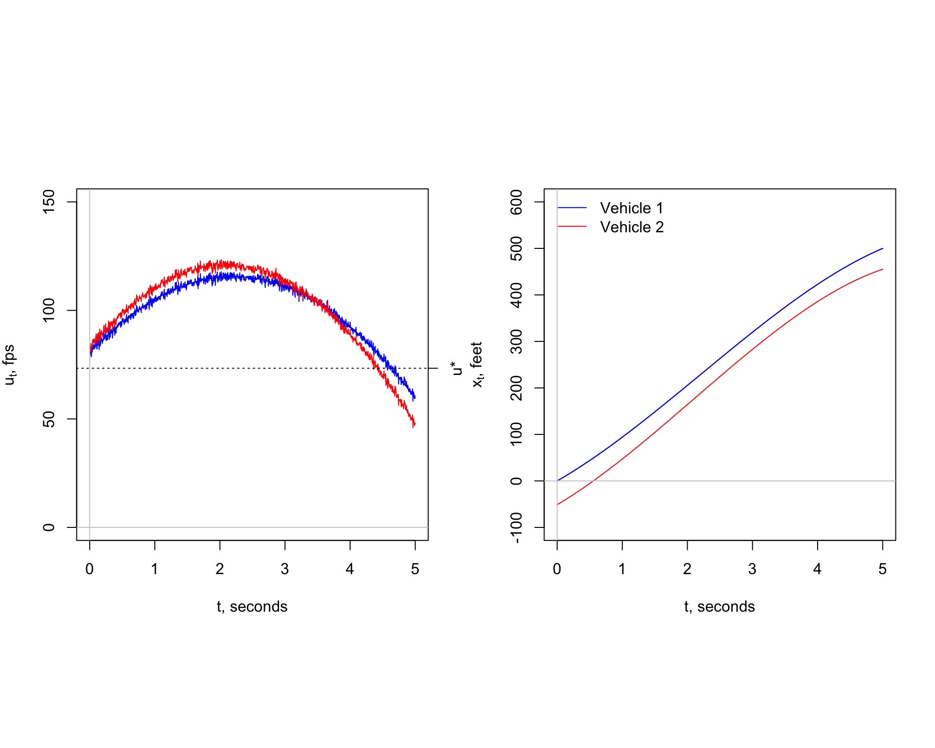
Since traffic is highly volatile, the first step is to simulate field conditions. We assume the traffic density is fixed, \(K = k\) = 50 vpm. Thus \(\bar{u} \pm \sigma = 41 \pm 11.6\) mph. Since \(X = 1 \rightarrow X = 0\), the speeds of the two vehicles before and after breakdown must satisfy the constraints \(u(t_{start}) > u^*\) and \(u(t_{end}) \le u^*\) where the time at the start and end of the simulation are \(t_{start}\) = 0 and \(t_{end}\) = 5 seconds. These values were estimated by drawing samples from a simulated data set consisting of one hundred draws from the normal distribution of \(N(\bar{u} = 41, \hat{\sigma}^2 = 11.6^2)\). Four draws were made from the simulated data. They are shown in the following table.

	Start	End
Time t	0	5 seconds
Vehicle 1: u	55 mph (81 fps)	41 mph (60 fps)
Vehicle 1: x	0 feet	500 feet
Vehicle 2: u	57 mph (83 fps)	32 mph (47 fps)
Vehicle 2: x	-68 feet	455 feet

Note that at the start of the simulation, \(t_{start} = 0\), that vehicle 2 is traveling at a speed slightly greater than vehicle 1. At the end of the simulation, \(t_{end}\) = 5 seconds, the opposite is true. The simulation also shows driver 2 is traveling at higher speed than driver 1 for the first three seconds. Driver 2 begins to decelerate around three seconds to maintain a safe headway at \(t_{end}\). Speed volatility explains these findings. Another simulation will be different.

The second step is to estimate model parameters \(a\) and \(b\) for each of the two vehicles. Other assumptions must be must made. The bottleneck is assumed tapper down from two to one lane in 500 feet and the total time for the breakdown is 5 seconds. The drivers are assumed to be risk averse so driver of vehicle 2 maintains a safe headway. All this information is summarized in the table. The \(t-x\) trajectory shows vehicle 2 maintains a safe headway for the entire 5 seconds of the simulation.

The same numerical integration scheme described earlier for determining \(x_t\) trajectories for the ring-road is used here. Like the ring-road, the \(t-x\) trajectories are smooth, suggesting the speeds at times \(t_0\) and \(t_{end}\) are more critical than the speed changes caused by Brownian motion \(W(t)\) ranging over the interval \(t_{start} < t < t_{end}\).

Traffic Breakdown Part 2

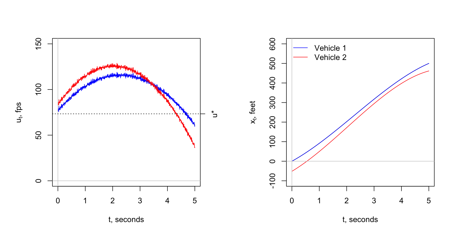
The importance of maintaining a safe headway cannot be overemphasized. Without this assumption, the \(t-x\) trajectory of vehicle 2 could cross the trajectory for vehicle 1. The result is a rear-end crash caused by tailgating. This possibility of a rear-end crash can occur even when there is a safe headway at \(t_{start}\) = 0 and \(t_{end}\) = 5. Let’s see.

The following simulation shows a near-miss caused by tailgating. While the trajectories do not cross, the \(t-x\) trajectories shows a safe headway violation between three and four seconds. Since drivers are assumed to risk averse, it is not unreasonable to assume the driver of the following vehicle will decelerate. In other words, not violate the safe headway assumption. To keep the discussion as simple as possible, the safe sight-line assumption for times \(0 < t < t_{end}\), discussed in the Bottleneck section, is not imposed here.

Traffic Breakdown Part 3

How is a traffic breakdown initiated in the first place? So far, we have tacitly assumed the lead vehicle decelerates from \(u_{start} > u^*\) and \(u_{end} < u^*\). Now we tackle a most challenging question. Instead of assuming to watch vehicles pass us from the road side, we will position ourselves overhead by analyzing photographs taken from a helicopter or drone flying overhead.

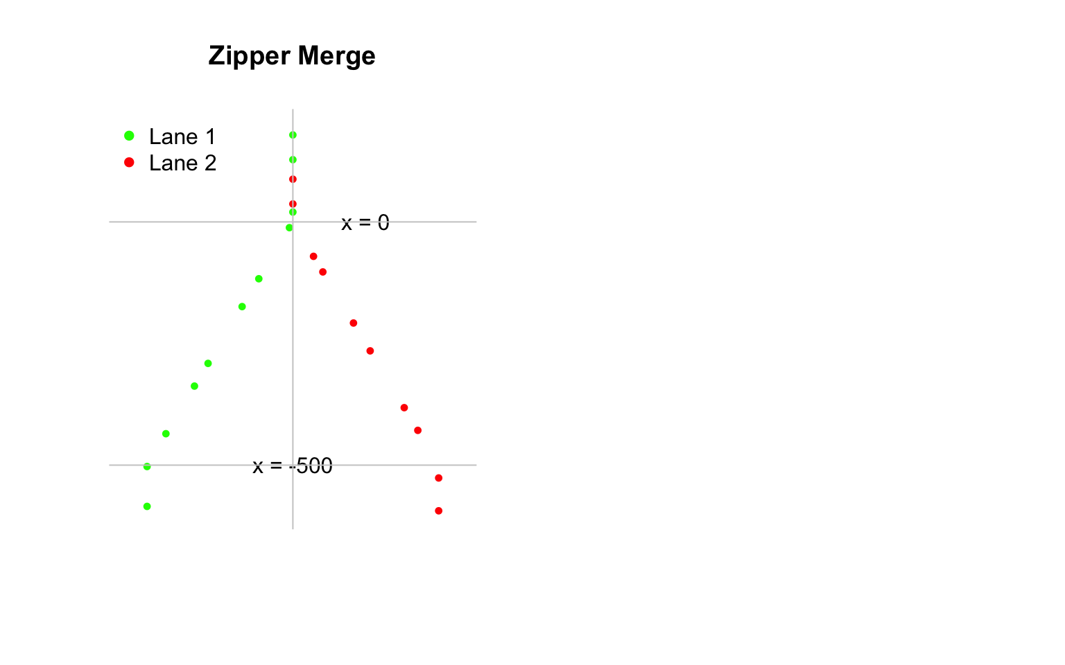
Here, the following graph shows two lanes of traffic merging into one lane. There is no traffic breakdown in this simulation. No queue forms. All drivers maintain free-flow speeds, \(u > u^*\) where \(u = \bar{u}\) = 55 mph. As above, we simulated speed using the \(U(k, a, b, h_{safe}, t)\) model. To maintain a \(X = 0\) state, all drivers of following vehicles keep a safe headway. This result is most vividly seen downstream where \(x > 0\) where the vehicles travel in one lane.

Since is controversy associated with the proper positioning of roadside equipment, it is interesting to note the following:

• \(Q = Q(x > 0) = Q(x \le 0)\)

because \(k\) = 50 vpm is a constant and \(\bar{u}\) is the same value both downstream and upstream of \(x = 0\). Thus, \(Q = k * \bar{u}\) where \(k = \frac{n}{l}\) and \(n\) is the total vehicle count obtained from the photo. A roadside collection of data taken any position on the photo downstream or upstream of \(x = 0\) gives the same result. We look at the controversy again after we answer the question: How is a traffic breakdown initiated in the first place?

Traffic Breakdown Part 4

The Zipper Merge graph demonstrates the importance of upstream vehicle alignment and the effects of noise of merging vehicle at a bottleneck over time. The spacing between vehicles is nonuniform and vehicle grouping is virtually impossible to predict.

A zipper merge is a special case because the upstream vehicles are aligned in a manner that it is unnecessary for vehicles to change speed. Now, we eliminate this assumption and put drivers under the stress by requiring a speed change of only one vehicle. Since our analysis takes place where the chance of a traffic breakdown is significant, \(k = 50\) vpm, the action of this driver may trigger a breakdown event causing a queue to form that moves upstream from \(x\) = 0.

To simplify the discussion, the effect of noise will be temporarily removed from the following “thought experiment.” This step may seem odd given the emphasis placed on stochastic modeling. After we complete the analysis, we will be in a better position to understand breakdown. More specifically, explaining and coming closer to reliably predicting the role that traffic noise plays in triggering breakdown. In other words, determine if traffic noise is a major or minor factor in explaining and predicting breakdown.

We will continue to observe vehicles from overhead. But this time, we will follow the actions of only two drivers, who are traveling side-by-side in lanes 1 and 2 at \(x = -500\) feet, the beginning of the merge section where freeway tappers down from two to one lane. The side-by-side vehicles, like the rest of the vehicles traveling in the direction of the bottleneck, are traveling at speed \(u\) = 55 mph. The driving scenario is similar to one described above before being transformed from a free-flow to congested state, \(X = 0 \rightarrow X = 1\).

Since the two drivers are side-by-side, one must make the decision to be the leader or follower. The choices are: (1) accelerate and merge and become a leader, or (2) decelerate and merge and become a follower. In either case, the drivers will do so safely. They will maintain a safe headway of at least \(h_{safe} = 53\) feet for speed of \(u\) = 41 mph. Most importantly and regardless of choice, the decision-maker does not want to disrupt the speeds of the other drivers, which are assumed to be traveling at \(u\) = 41 mph. The aim is to cause no further disruption or delay. In essence, the decision-maker wants to perform a zipper merge.

A series of photographs are taken for the two drivers in the two cases. Speed and location recordings are made every second over a period of 50 seconds. The data are analyzed and summarized as shown below in the \(y-x\) plots. Since the location \(x\) is measured in feet, speed \(u\) is shown in feet per second (fps).

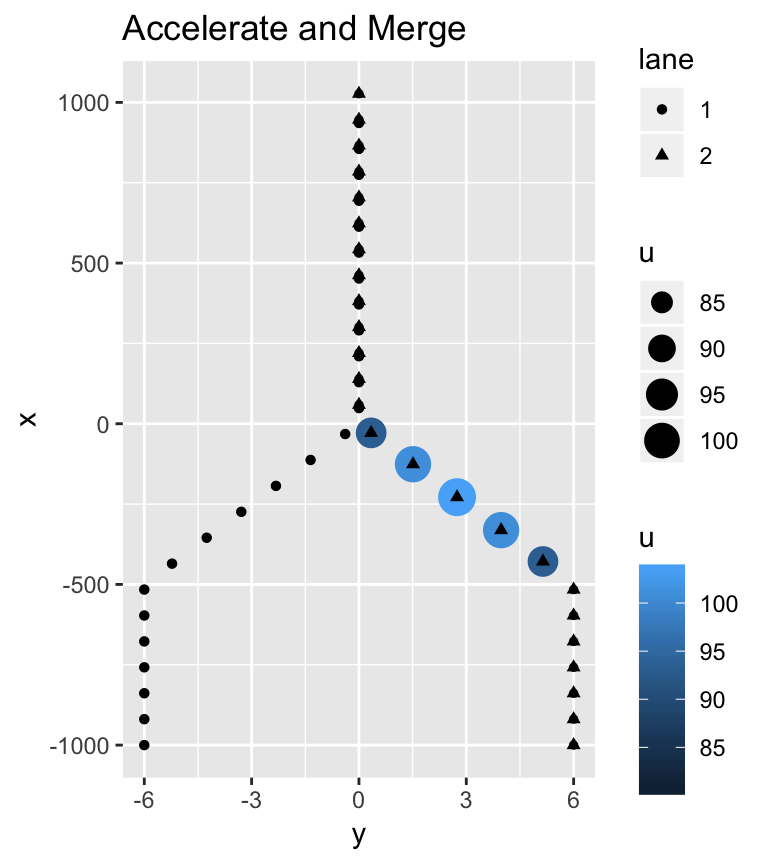
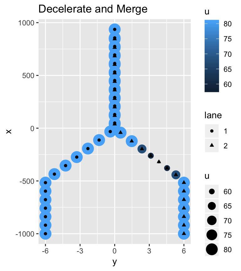
Regardless of the action taken, the aim of the decision-maker is achieved. The driver does not disturb the other drivers. No queue is formed. The accelerate and merge driver reaches a maximum speed of 50 mph (103 fps) and the decelerate and merge driver reaches a minimum speed of 40 mph (58 fps). The acceleration and deceleration rates are approximately equal to 7 and -7 ft/sec\(^2\), respectively. A maximum comfortable decelerate is considered to be 15 ft/sec\(^2\). Since all drivers are maintaining safe head-ways, no crash or near miss incidents are predicted.

---

References

Elefteriadou, Lily. 2014. An Introduction to Traffic Flow Theory. New York, New York: Springer.
Iacus, Stefano. 2008. Simulation and Inference for Stochastic Differential Equations: With R Examples. Springer-Verlag.
The cartools functions usdzipper, formqueue, freeflowpass passplot xabmerge3, brktrials3 and brkdelay are used to create the plots shown on this page.↩